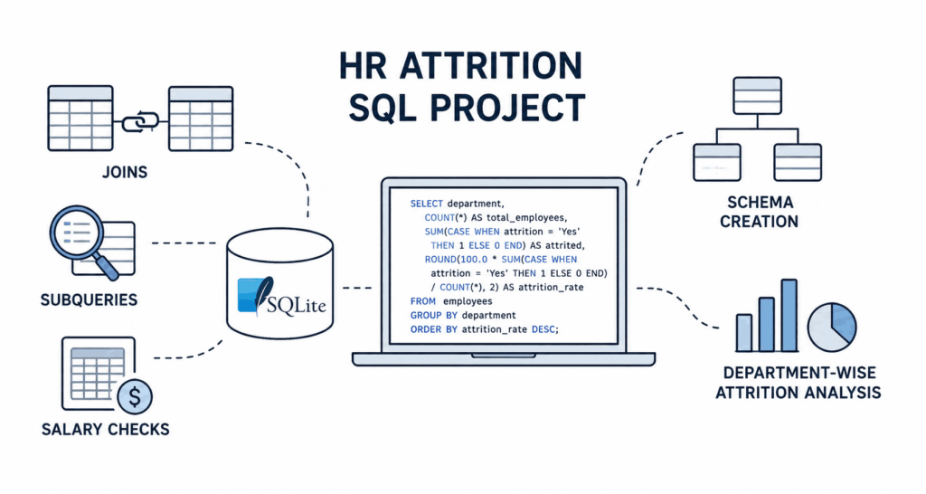
HR Queries & Attrition Check Using SQLite

SQL + HR Analytics Project

This HR Attrition SQL Project uses a Human Resources dataset inside SQLite to practice schema creation, joins, grouping, subqueries, salary checks, and department-wise attrition analysis. The notebook keeps the work direct and practical: load the data, shape it into useful tables, and answer HR questions using SQL.

About the project: The project starts by reading the HR CSV file in Kaggle, loading it into an in-memory SQLite database, and then breaking the raw table into smaller working tables such as employees, departments, salaries, and performance. After that, every task is solved with SQL queries written against those tables.

Data Source Human Resources dataset loaded from the Kaggle input directory.

Database Used SQLite in-memory database created directly inside the notebook.

Main SQL Skills JOIN, LEFT JOIN, GROUP BY, ORDER BY, LIMIT, HAVING, and subqueries.

Business Angle Salary ranking, performance checks, department averages, and attrition rate analysis.

Project Flow

Kaggle Input

→

Pandas DataFrame

→

SQLite Table

→

Schema Creation

→

HR SQL Queries

Tools and Libraries Used

Python Pandas NumPy SQLite3 Kaggle SQL Joins Subqueries HR Analytics

Notebook Steps and Code

Import Libraries and Check Kaggle Input Files

The notebook begins by importing basic Python libraries and printing the file path available inside the Kaggle input directory.

Python

import numpy as np 
import pandas as pd 
import os
for dirname, _, filenames in os.walk('/kaggle/input'):
    for filename in filenames:
        print(os.path.join(dirname, filename))

import kagglehub

Load the HR Dataset into SQLite

Here, the CSV is loaded into Pandas and then stored as an SQLite table named hr_data. A quick salary-based preview is also displayed.

Python + SQL

import sqlite3

csv_path = '/kaggle/input/datasets/rhuebner/human-resources-data-set/HRDataset_v14.csv'
df = pd.read_csv(csv_path)

conn = sqlite3.connect(':memory:')

df.to_sql('hr_data', conn, index=False, if_exists='replace')

query = """
    SELECT *
    FROM hr_data
    ORDER BY Salary DESC
    LIMIT 5;
"""

result_df = pd.read_sql_query(query, conn)
display(result_df)

Task 1: Create schema: employees, departments, salaries, performance tables and import data

This step breaks the original HR table into smaller tables. It makes the later JOIN queries cleaner and easier to understand.

Python + SQL

cursor = conn.cursor()

cursor.execute("DROP TABLE IF EXISTS departments;")
cursor.execute("""
    CREATE TABLE departments AS 
    SELECT DISTINCT DeptID, Department 
    FROM hr_data
    WHERE DeptID IS NOT NULL;
""")

cursor.execute("DROP TABLE IF EXISTS employees;")
cursor.execute("""
    CREATE TABLE employees AS 
    SELECT EmpID, Employee_Name, DeptID, ManagerID, ManagerName, Termd 
    FROM hr_data;
""")

cursor.execute("DROP TABLE IF EXISTS salaries;")
cursor.execute("""
    CREATE TABLE salaries AS 
    SELECT EmpID, Salary, Position 
    FROM hr_data;
""")


cursor.execute("DROP TABLE IF EXISTS performance;")
cursor.execute("""
    CREATE TABLE performance AS 
    SELECT EmpID, PerformanceScore, LastPerformanceReview_Date 
    FROM hr_data;
""")

conn.commit()

print("Schema successfully created! Ready for JOINs.")

View the Database Schema

After creating the schema, this block checks the tables and prints their column structure using SQLite metadata.

Python + SQLite Metadata

tables_query = """
    SELECT name 
    FROM sqlite_master 
    WHERE type='table' AND name != 'hr_data';
"""
tables_df = pd.read_sql_query(tables_query, conn)

print("📊 DATABASE SCHEMA OVERVIEW \n" + "="*30)

for table_name in tables_df['name']:
    print(f"\n📁 TABLE: {table_name.upper()}")
    print("-" * 30)
    
    pragma_query = f"PRAGMA table_info('{table_name}');"
    schema_df = pd.read_sql_query(pragma_query, conn)
    
    schema_summary = schema_df[['name', 'type', 'pk']].rename(columns={
        'name': 'Column Name',
        'type': 'Data Type',
        'pk': 'Is Primary Key?'
    })
    
    schema_summary['Is Primary Key?'] = schema_summary['Is Primary Key?'].astype(bool)
    
    display(schema_summary)

Task 2: INNER JOIN employee names and departments to list employee names with department name

This is the first proper JOIN task. It connects employee records with department names using the department ID.

SQL JOIN

query_2 = """
SELECT e.employee_name, d.department FROM employees e
JOIN Departments d ON d.deptid = e.deptID
"""

df_task2 = pd.read_sql_query(query_2, conn)
display(df_task2)

Task 3: LEFT JOIN to find employees with performance “Fully meets”

This query checks employee performance records and filters employees whose performance score is marked as Fully meets.

SQL LEFT JOIN

query_3 = """
SELECT Employee_Name from employees
left join PERFORMANCE on
employees.empID = PERFORMANCE.empID
WHERE PERFORMANCE.PerformanceScore LIKE "Fully meets"
"""

df_task3 = pd.read_sql_query(query_3, conn)
display(df_task3)

Task 4: Find department with highest average salary using JOIN + GROUP BY

This query joins departments, employees, and salaries, then groups salary values by department to find the highest average salary.

SQL GROUP BY

query_4 = """
    SELECT departments.department,
    avg(salaries.salary) as Highest
    FROM departments
    JOIN employees ON
    departments.deptID = employees.deptID
    JOIN salaries ON
    salaries.EmpID = employees.EmpID
    GROUP BY departments.department
    ORDER BY Highest Desc
    LIMIT 1
"""

df_task4 = pd.read_sql_query(query_4, conn)
display(df_task4)

Task 5: Subquery: find employees earning above department average salary

This task uses a subquery to compare each employee salary with the average salary of their own department.

SQL Subquery

query_5 = """
    SELECT employees.Employee_Name FROM employees
    JOIN salaries ON
    employees.EmpID = salaries.EmpID
    JOIN departments ON employees.DeptID = departments.DeptID
    WHERE salaries.salary > 
           (SELECT AVG(salaries.salary) FROM salaries
           JOIN employees ON
           salaries.empID = employees.empID
           WHERE
           departments.deptID = employees.deptID
           )
"""

df_task5 = pd.read_sql_query(query_5, conn)
display(df_task5)

Task 6: Join to calculate attrition rate per department (terminated/total)

This query calculates department-wise attrition rate by dividing terminated employees by total employees in each department.

SQL Attrition Rate

query_6 = """
    SELECT departments.department, ROUND((SUM(employees.termd)*100)/COUNT(employees.termd),2)
    FROM employees
    JOIN departments ON employees.deptID = departments.deptID
    GROUP BY departments.department
"""

df_task6 = pd.read_sql_query(query_6, conn)
display(df_task6)

Additional Attrition Check: Departments With Attrition Rate Above 20

The notebook ends by filtering departments where the calculated attrition rate is greater than 20.

SQL HAVING

query_7 = """
    SELECT departments.department, ROUND((SUM(employees.termd)*100)/COUNT(employees.termd),2) AS AR
    FROM employees
    JOIN departments ON employees.deptID = departments.deptID
    GROUP BY departments.department
    HAVING AR > 20
"""

df_task7 = pd.read_sql_query(query_7, conn)
display(df_task7)

Project insight: This notebook is useful because it treats HR data like a real business table, not just a file to preview. By separating the raw data into smaller tables and then writing joins, subqueries, and attrition checks, it shows how SQL can answer practical people analytics questions in a clean way.