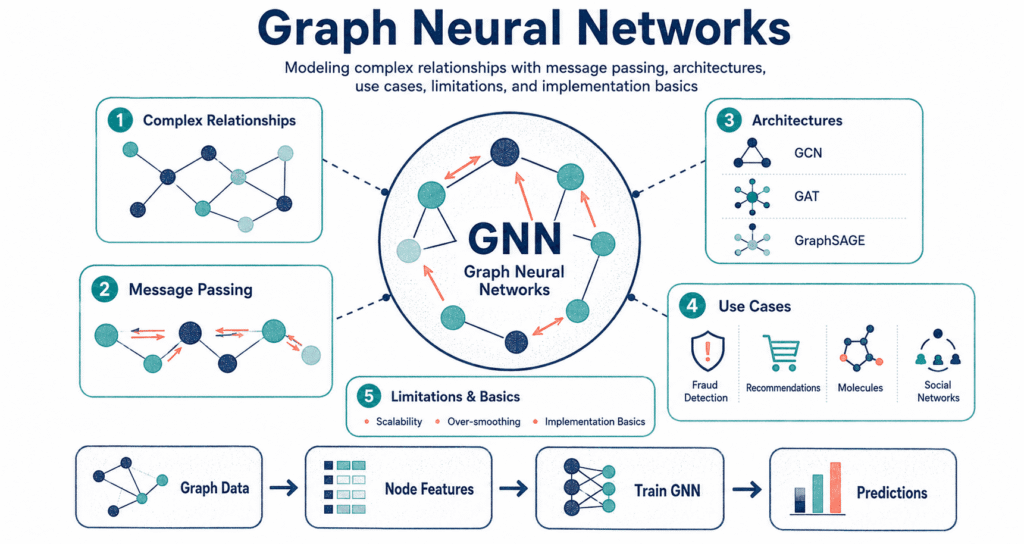
Graph Neural Networks (GNNs): Modelling Complex Relationships

Why Graph Neural Networks Matter

Many real-world datasets are not naturally flat. A social network is not just a list of users. It is a web of friendships, followers, communities, and influence paths. A molecule is not just a collection of atoms. It is a structure where bonds determine chemical behaviour. A fraud network is not just individual transactions. It is a pattern of accounts, devices, merchants, and repeated connections.

Standard machine learning models usually expect a table: rows as examples and columns as features. That format is useful, but it often destroys relational information. If two accounts are linked through a chain of suspicious transfers, a flat model may not easily see that network pattern unless we manually engineer complex features.

Graph Neural Networks solve this problem by learning directly from graph structure. They combine node attributes with neighbourhood information. As a result, a node’s prediction can be influenced not only by its own features, but also by the features and structure around it.

What Is a Graph?

A graph is a mathematical structure used to represent objects and relationships. The objects are called nodes or vertices. The relationships are called edges or links. Edges can be directed or undirected, weighted or unweighted, homogeneous or heterogeneous.

In an undirected graph, the connection works both ways. A friendship relation is often treated this way. In a directed graph, the relationship has direction. A follows B does not always mean B follows A. In a weighted graph, edges have strength, cost, frequency, distance, or confidence attached.

Graphs become especially useful when the relationship itself carries predictive signal. For example, in recommendation systems, users connected to similar products may have similar preferences. In citation networks, papers connected by references may share topics. In traffic networks, roads connected to congested roads may soon experience congestion.

Why Traditional Models Struggle with Graph Data

Traditional models assume that each row is mostly independent. This works well for many problems, but graph data violates that assumption. In a graph, one node’s meaning may depend heavily on its neighbours. A user may look normal alone but suspicious when connected to a cluster of known fraudulent accounts.

Another issue is variable structure. Images have a fixed grid. Text has a sequence. Tables have columns. Graphs can have any number of nodes, any number of edges, and irregular neighbourhood sizes. One node may have two neighbours, while another may have two million.

Because of this irregularity, we need models that can handle variable neighbourhoods and remain insensitive to arbitrary node ordering. If we rename node 1 as node 50, the meaning of the graph should not change. GNNs are designed around this requirement.

The Core Idea: Message Passing

The central mechanism in most Graph Neural Networks is message passing. Each node gathers information from its neighbours, combines those messages, and updates its own representation. After one layer, a node knows about its immediate neighbours. After two layers, it can receive information from neighbours of neighbours.

This is powerful because many relationships are not direct. In a social network, your friend’s friend may belong to a community relevant to you. In fraud detection, a suspicious account may not connect directly to a known fraudster but may share devices, merchants, or transfer chains through intermediate nodes.

The aggregation step must handle any number of neighbours. Common aggregators include sum, mean, max, and attention-weighted combinations. The update step is usually a neural network operation that transforms the old node representation and the aggregated neighbourhood information into a new embedding.

Node, Edge, and Graph-Level Tasks

Graph Neural Networks can be used for different prediction levels. The right task depends on what you want to predict. Sometimes the target is a node. Sometimes it is an edge. Sometimes it is the entire graph.

Node-level prediction answers questions about individual entities. For example, classify a paper by research topic, detect whether an account is risky, or predict a user segment. Edge-level prediction answers questions about relationships. For example, will a user buy a product, will two proteins interact, or is a transaction suspicious? Graph-level prediction answers questions about the whole structure, such as whether a molecule has a desired property.

Popular GNN Architectures

GNN is a broad family, not one single model. Different architectures define different ways of aggregating neighbour information and updating node embeddings. Three important ideas are Graph Convolutional Networks, GraphSAGE, and Graph Attention Networks.

Graph Convolutional Networks, often called GCNs, popularized an efficient way to apply neural networks directly to graph-structured data. A GCN layer mixes information from connected nodes using a normalized version of the graph adjacency structure.

GraphSAGE focuses on inductive learning. Instead of learning a separate embedding for every node, it learns an aggregation function that can generate embeddings for unseen nodes. This is valuable when new users, products, devices, or documents arrive after training.

Graph Attention Networks, or GATs, use attention to weigh neighbours differently. This is useful because not all neighbours are equally important. In a fraud graph, a high-risk shared device may matter more than a weak connection to a normal merchant.

Graph Embeddings: The Output of Representation Learning

A major goal of Graph Neural Networks is to create embeddings. An embedding is a dense numerical representation that captures useful information. In a GNN, a node embedding can encode both the node’s own attributes and the structure around it.

These embeddings can then be used for prediction. A classifier can use node embeddings to predict labels. A similarity function can compare user and product embeddings for recommendation. A graph embedding can represent an entire molecule, transaction chain, or document network.

This is similar in spirit to word embeddings in NLP or image embeddings in computer vision. The difference is that graph embeddings must respect relationship structure. The model learns not only what a node is, but also where it sits in the network.

A Small PyTorch Geometric Example

In practice, most developers use libraries instead of implementing GNN layers from scratch. PyTorch Geometric is a popular library for building and training Graph Neural Networks with PyTorch. It represents a graph using tensors such as node features and edge indices.

The following example shows the basic shape of a two-layer GCN model. It is intentionally compact. The goal is to show how graph structure enters the model through edge_index while node features enter through x.

import torch
import torch.nn.functional as F
from torch_geometric.nn import GCNConv

class SimpleGCN(torch.nn.Module):
    def __init__(self, num_features, hidden_channels, num_classes):
        super().__init__()
        self.conv1 = GCNConv(num_features, hidden_channels)
        self.conv2 = GCNConv(hidden_channels, num_classes)

    def forward(self, x, edge_index):
        # x: node feature matrix [num_nodes, num_features]
        # edge_index: graph connectivity [2, num_edges]
        x = self.conv1(x, edge_index)
        x = F.relu(x)
        x = F.dropout(x, p=0.5, training=self.training)
        x = self.conv2(x, edge_index)
        return x

model = SimpleGCN(
    num_features=16,
    hidden_channels=32,
    num_classes=3
)

A real project would include data loading, train-validation-test masks, optimizer setup, loss calculation, and evaluation. However, the core pattern remains the same: node features and graph connectivity flow together through graph convolution layers.

Where Graph Neural Networks Are Used

GNNs are useful when relationships are central to the problem. They are common in recommendation systems, fraud detection, molecular property prediction, traffic forecasting, knowledge graphs, cybersecurity, social network analysis, and supply chain modelling.

In recommendation systems, a graph can connect users, products, categories, searches, purchases, ratings, and sessions. A GNN can learn from these relationships to recommend products that are not obvious from user attributes alone.

In fraud detection, suspicious activity often appears as network structure. Multiple accounts may share devices, phone numbers, addresses, cards, or transaction patterns. GNNs can help detect suspicious clusters and indirect relationships that traditional models may miss.

In drug discovery, molecules can be represented as graphs where atoms are nodes and bonds are edges. A GNN can learn how molecular structure relates to properties such as toxicity, solubility, or binding behaviour.

In traffic forecasting, roads, intersections, stations, or sensors can be represented as nodes, while physical connections become edges. A GNN can combine local sensor features with network structure to model congestion propagation.

GNNs and Complex Relationships in Business Problems

Graph Neural Networks are not only academic models. They are also useful for business analytics when relationships drive outcomes. Many customer, supply, risk, and operations problems are network problems in disguise.

Consider a bank trying to detect mule accounts. A single account may not look risky based on transaction amount alone. But if it connects to several accounts already flagged as suspicious, uses the same device fingerprints, and participates in short-lived transfer chains, the graph context becomes highly informative.

Similarly, in B2B sales, company relationships can matter. One customer may be connected to parent companies, subsidiaries, suppliers, partners, and competitors. A graph model can capture these links and support lead scoring, churn prediction, or account prioritization.

This connects naturally with anomaly detection. When anomalies appear as unusual relationships rather than unusual individual rows, graph-based learning becomes valuable. For a broader view of anomaly modelling, see Codeayan’s guide on anomaly detection in high-dimensional data.

Homogeneous vs Heterogeneous Graphs

A homogeneous graph has one type of node and one type of edge. A citation graph with papers connected by citations can be treated as homogeneous. This makes modelling simpler because every node and edge has the same semantic role.

Many real-world systems are heterogeneous. An e-commerce graph may contain users, products, brands, categories, sellers, orders, reviews, and search queries. The edges may represent purchases, views, reviews, belongs-to, ships-from, or searches-for. Treating every node and edge as the same can lose meaning.

Heterogeneous GNNs handle different entity and relationship types more carefully. They can learn relation-specific transformations and preserve semantic differences. This is important in enterprise graphs, knowledge graphs, and recommendation systems.

Common Challenges in GNN Projects

GNNs are powerful, but they are not automatically better than simpler methods. The first challenge is data construction. Building the graph is often harder than training the model. You must decide what becomes a node, what becomes an edge, what features to attach, and what time window to use.

The second challenge is scalability. Large graphs can have millions or billions of edges. Full-batch training may become impossible. Sampling, mini-batching, distributed training, and efficient storage become important.

The third challenge is evaluation. Random splits can create leakage in graph problems. If future edges appear in training, or if connected entities are split carelessly, the model may look better than it really is. Time-based validation is often necessary in fraud, recommendation, and transaction networks.

Another challenge is oversmoothing. When too many GNN layers are stacked, node embeddings can become too similar. The model may lose useful distinctions between nodes. Deeper is not always better in GNNs.

• Graph construction: poor node and edge definitions can ruin the project.
• Scalability: large graphs require sampling and efficient training pipelines.
• Leakage: graph splits must respect time, entities, and real deployment conditions.
• Oversmoothing: too many layers can make node representations indistinguishable.
• Explainability: understanding why a GNN made a prediction can be difficult.

Explainability in Graph Neural Networks

GNN explainability is important because graph predictions often affect risk, recommendation, security, and scientific decisions. Stakeholders may want to know which neighbours, edges, paths, or subgraphs influenced the prediction.

Explainability is harder in GNNs than in many tabular models because the prediction depends on both features and structure. A node may be classified as risky because of its own attributes, because of one important neighbour, or because of a larger pattern around it.

Practical explanations often focus on important features, influential neighbours, high-impact edges, or small subgraphs that contributed to a decision. For a broader introduction to model interpretability, Codeayan’s guide on Explainable AI is a useful companion topic.

How to Start a GNN Project

Start with the problem, not the model. Ask whether relationships are truly important. If a simple tabular model using engineered relationship features performs well, a GNN may not be necessary. GNNs are most useful when relational structure carries unique signal.

Next, define the graph schema. Decide what the node types are, what the edge types are, whether edges are directed, whether they need weights, and whether time matters. Then create features for nodes and edges. Raw IDs alone are usually not enough.

After that, build a baseline. A non-GNN baseline is valuable because it tells you whether the graph model is actually adding value. Compare against logistic regression, random forest, gradient boosting, or matrix factorization depending on the task.

Best Practices for Modelling Complex Relationships

Good GNN projects depend on careful design choices. Do not add every possible edge just because data is available. Edges should represent meaningful relationships. Too many weak or noisy edges can make message passing less useful.

Use time-aware validation whenever the graph evolves. If a model will predict future fraud, train on past data and test on future data. If a recommender will serve new users, evaluate whether the model handles unseen nodes or only memorizes existing relationships.

Keep model depth reasonable. Many successful GNNs use only a few layers. If you need long-range information, consider better graph construction, sampling strategies, residual connections, attention, or task-specific architecture changes rather than simply adding layers.

• Define meaningful edges: relationships should represent real signal, not random availability.
• Use strong baselines: prove the GNN adds value over simpler methods.
• Respect time: avoid future information leaking into training.
• Monitor scalability: graph size can grow faster than expected.
• Check explainability: inspect which neighbours or subgraphs influence predictions.
• Plan deployment early: online graphs, new nodes, and changing edges need careful handling.

GNNs vs Other Deep Learning Models

Convolutional Neural Networks are strong for grid-like data such as images. Recurrent and transformer models are strong for sequences such as text. Graph Neural Networks are designed for irregular relational structures where connections are part of the input.

This does not mean GNNs replace other models. In many systems, they complement them. A document can be encoded with a transformer, while citations between documents are modelled with a GNN. An image can be processed with a CNN, while detected objects and scene relationships form a graph.

Modern AI systems often combine multiple representations. The best architecture depends on whether the strongest signal is visual, textual, tabular, temporal, or relational. GNNs become important when the relational signal is too valuable to ignore.

Deployment Considerations

Deploying a GNN can be more complex than deploying a standard classifier. In a tabular model, you send one row of features and receive one prediction. In a GNN, prediction may require neighbourhood information, graph sampling, current edges, and updated node embeddings.

Some systems precompute embeddings offline and use them in a downstream model. Others perform online neighbourhood lookup at prediction time. Offline embeddings are simpler and faster, but may become stale. Online graph inference is fresher, but more expensive and operationally complex.

Model compression may also matter if GNN outputs are used in production systems with strict latency requirements. For related deployment efficiency ideas, Codeayan’s article on model quantization and distillation provides useful context.

Common Mistakes to Avoid

The first mistake is using a GNN because the topic sounds advanced. If the graph structure does not add meaningful signal, a GNN may increase complexity without improving results.

The second mistake is building the graph carelessly. Node and edge definitions are modelling decisions. A bad graph can make a good model fail. For example, connecting users only because they visited the same popular page may create noisy relationships that hide stronger signals.

The third mistake is evaluating with unrealistic splits. If the model sees future relationships during training, performance will be inflated. This is especially dangerous in recommendation, fraud, cybersecurity, and temporal networks.

• Do not assume every relational dataset needs a GNN.
• Do not create edges without clear meaning.
• Do not ignore edge direction, weights, or time.
• Do not compare only against weak baselines.
• Do not evaluate with random splits when the real task is time-based.

Key Takeaways

Conclusion

Further reading: Review the Graph Convolutional Networks paper, Graph Attention Networks paper, GraphSAGE paper, and the PyTorch Geometric documentation.